Snowflake Secret#
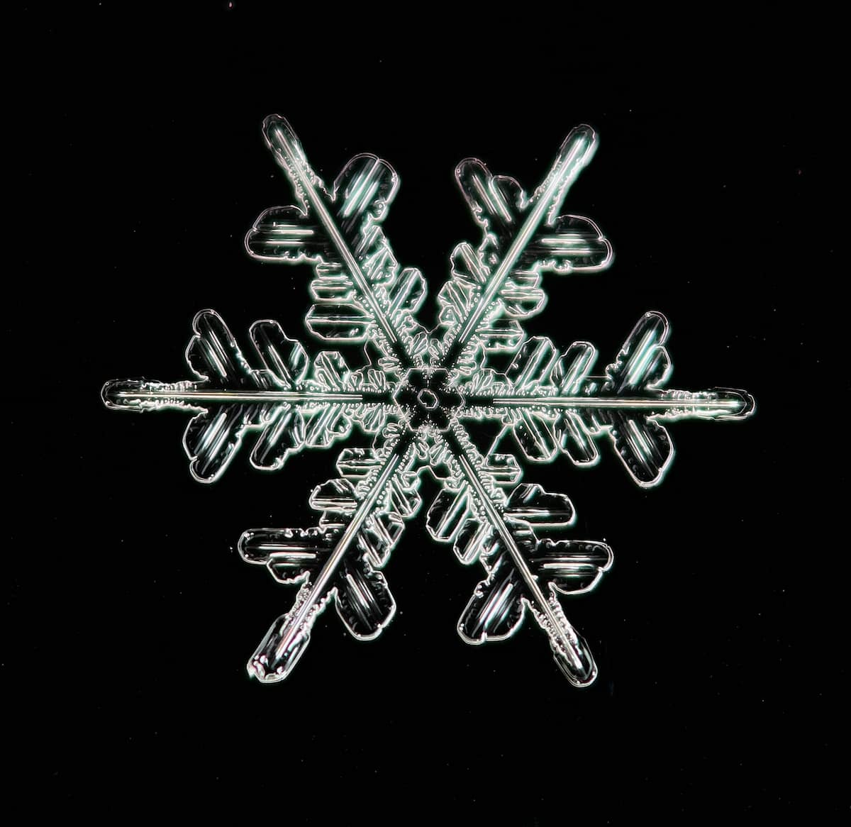
Fig. 3 Snowflake Photo by Zdeněk Macháček on Unsplash#
The Enchanting Tale of Fractals#
For centuries, the captivating complexity of fractals shapes with endless detail repeating at ever-smaller scales, existed as a mathematical curiosity. However, it wasn’t until the arrival of computers in the mid-20th century that fractals truly blossomed. Pioneering mathematicians like Felix Hausdorff laid the groundwork with concepts like fractal dimension, but it was Benoit Mandelbrot who revolutionized the field. Armed with the computational power of computers, Mandelbrot could finally visualize these intricate structures in stunning detail.
These eye-catching visuals, impossible to render by hand, brought fractals to life, igniting widespread fascination and propelling them from obscure mathematical concept to a captivating scientific phenomenon. This newfound ability to see the beauty of fractals fueled a surge in research, revealing self-similar patterns everywhere – from coastlines and snowflakes to the branching of trees and the vastness of the cosmos (See this source).
One fascinating aspect of fractals is their dimensionality. Unlike traditional geometric shapes, which have integer dimensions (a line is 1D, a square is 2D, a cube is 3D), fractals can have non-integer dimensions. This unusual property arises from their infinite complexity and self-similarity.
Another intriguing concept is the use of initiators and generators in creating fractals. An initiator is a starting shape, and a generator is an arranged collection of scaled copies of the initiator. Through a process of recursion, where the initiator is repeatedly replaced with the generator, we can create intricate fractal patterns.
One of the most striking examples of fractals in nature is the Romanesco broccoli. This unique vegetable showcases a fractal pattern in its florets. Each bud is composed of a series of smaller buds, all arranged in a logarithmic spiral. This self-similar pattern continues at smaller levels, giving a form approximating a natural fractal. The Romanesco broccoli is a testament to the pervasive presence of fractals in our natural world, reminding us of the hidden mathematical beauty in our everyday surroundings.
Today, fractals remain a dynamic field of study, with applications reaching far beyond pure mathematics, influencing computer graphics, engineering, and even financial modeling. In the same spirit of exploration and visualization, Python empowers us to create similar captivating visuals of these intricate shapes. With a few lines of code, we can embark on our own journey into the mesmerizing world of fractals, just like the mathematicians who first unveiled their hidden beauty.
Tip
Fractals are geometric marvels with intricate patterns that repeat endlessly at smaller scales. Whether it’s the jagged outline of a coastline, the delicate symmetry of a snowflake, or the branching form of a cauliflower, the same fundamental structure recurs in increasingly finer detail. This remarkable property, known as self-similarity, is the essence of fractals, making them both mesmerizing and profound in their complexity.
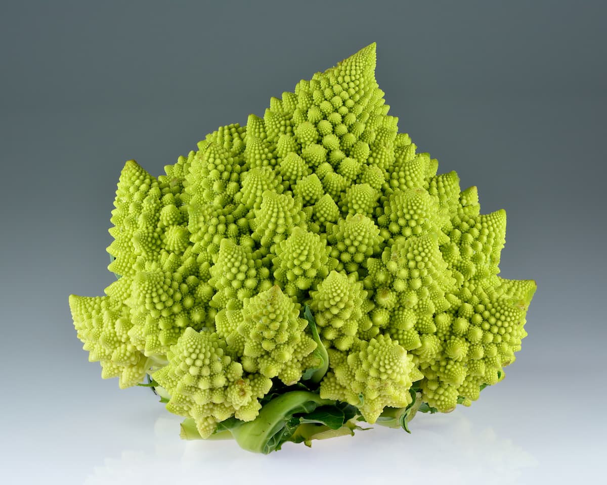
Fig. 4 The Romanesco broccoli is a surprising example of a fractal in nature. Its florets spiral outwards in a repeating pattern, where each floret resembles a miniature version of the entire head, showcasing a fascinating self-similar complexity (Ivar Leidus, CC BY-SA 4.0, via Wikimedia Commons)#
Conjuring Fractals: A Pythonic Tale#
Let’s get our hands dirty to create a fascinating fractal known as the Koch Snowflake. Python, the sorcerer of scientific computing, empowers us to visualize beautiful fractals with powerful tools like NumPy and Matplotlib in an exciting way. This journey begins with a seemingly simple line, a humble beginning. But as we delve deeper, this line undergoes a series of magical transformations, crystallizing into the intricate and beautiful snowflake. Named after the Swedish mathematician Helge von Koch, this fractal is a marvel of self-similarity: no matter how closely you zoom in, each part mirrors the whole. This process not only unveils the elegance of fractals but also provides a fantastic learning experience.
Our journey will take us through:
-
Visualizing Geometric Shapes: Python empowers us to translate abstract mathematical concepts into captivating visuals, allowing us to perceive and comprehend geometric shapes in a new light.
-
Mastering Manipulations: We’ll create functions to segment lines, rotate points, and translate or reflect shapes. These manipulations, akin to spells, become the building blocks for creating complex fractal structures.
-
Witnessing Mathematical Transformations: Experience the power of mathematics firsthand as we apply transformations repeatedly. Each iteration builds upon the previous one, revealing the captivating self-similar nature of fractals!
The Koch snowflake, with its intricate branching patterns and infinite detail, is a captivating example of a fractal. But how do we create this mesmerizing shape using Python? It’s easy; we’ll do it one step at a time.
The Building Blocks:
-
Line Segment Breakdown: Our journey begins with a simple line segment. We’ll divide this line into three equal parts using four equally spaced points, setting the stage for the transformation to come.
-
Rotation: To achieve the characteristic branching of the snowflake, we’ll need to rotate specific points on the line segment. This is where a rotation matrix comes in. Rotation matrices are mathematical tools that allow us to precisely rotate points around a specific origin.
-
Recursion: The Koch snowflake’s beauty lies in its self-similar nature. We’ll achieve this using a powerful technique called recursion. Recursion involves a function calling itself with progressively smaller versions of the initial problem. In our case, the function will generate smaller and smaller line segments with the snowflake’s branching pattern, ultimately forming the final shape.
-
Geometric Transformations: After generating the line fractal using recursion, we’ll apply additional geometric transformations like rotation and reflection. These transformations add complexity and create the final snowflake form.
Let’s Begin!
Now that we have a roadmap for creating the Koch snowflake, it’s time to import the necessary libraries and dive into the code. As we progress, we’ll explore essential concepts step-by-step.
Show code cell source
# Importing necessary libraries:

# NumPy for numerical computations
import numpy as np

# Matplotlib libraries for visualization
import matplotlib.animation as animation  # for animation
import matplotlib.pyplot as plt

# Matplotlib patch for drawing curved segments (arcs)
from matplotlib.patches import Arc

# Using random numbers
import random

# Interactive widgets library for Jupyter Notebooks
import ipywidgets as widgets

# Display library for Jupyter Notebooks
from IPython.display import display
Welcome to the Matrix#
In this project, we rely on NumPy’s powerful capabilities to streamline our fractal generation process. Here’s how NumPy supercharges our workflow:
-
Efficient Data Management: Fractals deal with massive amounts of data. NumPy stores and manipulates it with lightning speed, making calculations and memory usage more efficient.
-
Vectorized and Iterative Operations: Forget tedious loops. NumPy allows us to apply transformations and perform iterative computations on entire sets of data at once, boosting performance and making the code cleaner and more concise.
-
Seamless Visualization: NumPy integrates smoothly with Matplotlib, facilitating easy and efficient visualization of our fractal patterns.
Leveraging the combined strengths of NumPy and Matplotlib yields faster code, enhanced readability, and captivating visualizations that breathe life into our fractals.
A crucial step in crafting our mesmerizing snowflake is the ability to rotate points around an origin. This is achieved through a rotation matrix, which utilizes trigonometric functions (sine and cosine) to calculate a point’s new position after a specified rotation angle. Let’s define a Python function to handle this task. It will accept a point as a NumPy array with x and y coordinates and the desired rotation angle (in degrees). The function will convert the angle to radians, construct a 2x2 rotation matrix, and multiply it with the point to determine the new, rotated coordinates.
Show code cell source
def rotate_point_around_origin(point: np.array, angle_degrees: float) -> np.array:
    """
    Rotate a point around the origin by a given angle in degrees.

    Parameters:
    point (np.array): The point to be rotated, represented as a 2D numpy array [x, y].
    angle_degrees (float): The angle of rotation in degrees.

    Returns:
    np.array: The rotated point, represented as a 2D numpy array [x', y'].
    """
    angle_radians = np.radians(angle_degrees)
    rotation_matrix = np.array(
        [
            [np.cos(angle_radians), -np.sin(angle_radians)],
            [np.sin(angle_radians), np.cos(angle_radians)],
        ]
    )
    return np.dot(rotation_matrix, point)
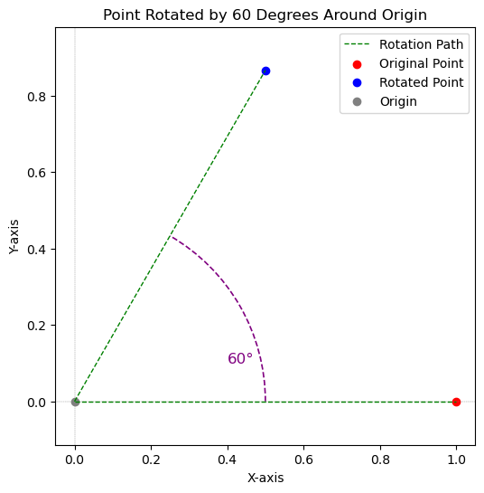
Example 1: Point Rotation#
Show code cell source
# Define a point to rotate
point = np.array([1, 0])  # This represents a point at (1, 0)

# Choose an angle of rotation
angle_degrees = 60

# Rotate the point using the function
rotated_point = rotate_point_around_origin(point, angle_degrees)

# Plot the points for visualization
plt.figure(figsize=(6, 6))  # Set figure size for better visualization

# Draw origin and point lines (dashed for reference)
plt.axhline(y=0, color='gray', linestyle='--', linewidth=0.3)
plt.axvline(x=0, color='gray', linestyle='--', linewidth=0.3)
plt.plot([0, 1], [0, 0], color='green', linestyle='--', linewidth=1)
plt.plot([0, rotated_point[0]], [0, rotated_point[1]], color='green', linestyle='--', linewidth=1, label='Rotation Path')

# Plot the points
plt.scatter(point[0], point[1], color="red", marker='o', label="Original Point")
plt.scatter(rotated_point[0], rotated_point[1], color="blue", marker='o', label="Rotated Point")
plt.scatter(0, 0, color="gray", marker='o', label="Origin")

# Draw an arc to show the rotation angle
arc = Arc((0, 0), 1, 1, theta1=0, theta2=angle_degrees, edgecolor='purple', linestyle='--', linewidth=1.2)
plt.gca().add_patch(arc)

# Add text to indicate the angle
plt.text(0.4, 0.1, f'{angle_degrees}°', fontsize=12, color='purple')

# Add labels and title
plt.xlabel("X-axis")
plt.ylabel("Y-axis")
plt.title(f"Point Rotated by {angle_degrees} Degrees Around Origin")

# Add legend
plt.legend()

# Set equal aspect ratio for a circular plot
plt.axis('equal')

# Show the plot
plt.show()
Tip
Rotation matrices are essential tools for 2D transformations, encoding the relationship between a point’s original and rotated positions. The 2D rotation matrix is given by:
Here, \(\theta\) is the rotation angle in radians. Multiplying this matrix by a point’s coordinates as a 2D NumPy array (e.g., [x, y]) yields the rotated coordinates. This concept is fundamental for many graphical transformations.
Sculpting the Curve#
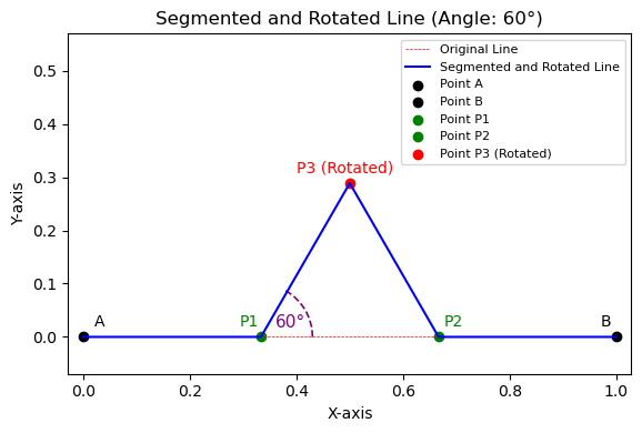
As we construct the Koch snowflake, we require to forge its foundational elements. Let’s define a function that serves two essential purposes:
-
Line Segmentation:
-
For the Koch snowflake, we divide a line segment into four equally spaced points: A, P1, P2, and B.
-
These points partition the line segment into three equal parts.
-
Points P1 and P2 are positioned at distances of 1/3 and 2/3 from point A to point B, respectively.
-
-
Point Rotation:
-
With our segmented line, we proceed to rotate one of the points around another point.
-
We select point P1 as the center of rotation.
-
Point P2 is then rotated around P1 by a specified angle (\(\theta\)).
-
This rotation is executed using the rotation function we previously defined.
-
The resulting point, denoted as P3, becomes part of the new modified shape.
-
Through recursive application of these steps to each smaller segment, we can construct the intricate shape known as the Koch curve.
Show code cell source
def break_and_rotate_line(x_values: np.array, y_values: np.array, angle: float) -> tuple:
    """
    Break a line into segments, rotate one point, and return points in specified order.

    Parameters:
    x_values (np.array): The x-coordinates of the endpoints of the line.
    y_values (np.array): The y-coordinates of the endpoints of the line.
    angle (float): The angle by which to rotate the third point of the line.

    Returns:
    tuple: The x and y coordinates of the points on the broken and rotated line.
    """
    # Calculate the line points
    x_points = np.linspace(x_values[0], x_values[1], 4)
    if np.isclose(x_values[0], x_values[1], atol=1e-8):
        y_points = np.full(4, y_values[0])
    else:
        coefficients = np.polyfit(x_values, y_values, 1)
        slope = coefficients[0]
        intercept = coefficients[1]
        y_points = slope * x_points + intercept
    # Rotate the third point around the second point by the given angle
    A = np.array([x_points[1], y_points[1]])
    B = np.array([x_points[2], y_points[2]])
    rotated_B = rotate_point_around_origin(B - A, angle) + A
    # Insert the rotated point after the second point
    x_points = np.insert(x_points, 2, rotated_B[0])
    y_points = np.insert(y_points, 2, rotated_B[1])

    return x_points, y_points
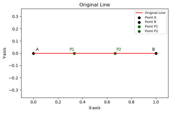
Example 2: Breaking the Line#
Show code cell source
# Define an initial line segment
x_values = np.array([0, 1])  # Line from (0, 0) to (1, 0)
y_values = np.array([0, 0])  # Horizontal line

# Angle of rotation (experiment with different values!)
angle = 60

# Break and rotate the line segment
new_x_points, new_y_points = break_and_rotate_line(x_values, y_values, angle)

# Extract point coordinates for clarity
A = np.array([new_x_points[0], new_y_points[0]])  # Point A (start)
B = np.array([new_x_points[4], new_y_points[4]])  # Point B (end)
P1 = np.array([new_x_points[1], new_y_points[1]])  # Point P1 (second point)
P2 = np.array([new_x_points[3], new_y_points[3]])  # Point P2 (third point)
P3 = np.array([new_x_points[2], new_y_points[2]])  # Point P3 (rotated point)

# --- Plot the Original Line (Figure 1) ---
plt.figure(figsize=(6, 4))  # Create a new figure for the original line
plt.plot(x_values, y_values, color='red', label='Original Line')

# Plot points on the original line and add annotations (offset slightly)
plt.scatter(A[0], A[1], marker='o', color='black', label='Point A')
plt.annotate("A", A + [0.02, 0.02], color='black', fontsize=10)
plt.scatter(B[0], B[1], marker='o', color='black', label='Point B')
plt.annotate("B", B + [-0.03, 0.02], color='black', fontsize=10)
plt.scatter(P1[0], P1[1], marker='o', color='darkgreen', label='Point P1')
plt.annotate("P1", P1 + [-0.04, 0.02], color='darkgreen', fontsize=10)
plt.scatter(P2[0], P2[1], marker='o', color='darkgreen', label='Point P2')
plt.annotate("P2", P2 + [0.01, 0.02], color='darkgreen', fontsize=10)

plt.xlabel("X-axis")
plt.ylabel("Y-axis")
plt.title(f"Original Line")
plt.axis('equal')
plt.xlim([-0.1, 1.1])  # Set limits for better visualization
plt.ylim([-0.1, 0.1])  # Adjust y-limits for horizontal line
plt.legend(fontsize=8)
plt.tight_layout()  # Adjust spacing to avoid label clipping

# --- Plot the Segmented and Rotated Line (Figure 2) ---
plt.figure(figsize=(6, 4))  # Create a new figure for the rotated line
plt.plot(x_values, y_values, color='red', label='Original Line', linestyle='--', linewidth=0.5)
plt.plot(new_x_points, new_y_points, color='blue', label='Segmented and Rotated Line')

# Add text to indicate the angle
plt.text(0.36, 0.018, f'{angle}°', fontsize=11, color='purple')

# Draw an arc to show the rotation angle
arc = Arc((0.33, 0), 0.2, 0.2, theta1=0, theta2=angle, edgecolor='purple', linestyle='--', linewidth=1.2)
plt.gca().add_patch(arc)

# Add point labels and annotations (optional, adjust positions if needed)
plt.scatter(A[0], A[1], marker='o', color='black', label='Point A')
plt.scatter(B[0], B[1], marker='o', color='black', label='Point B')
plt.scatter(P1[0], P1[1], marker='o', color='green', label='Point P1')
plt.scatter(P2[0], P2[1], marker='o', color='green', label='Point P2')
plt.scatter(P3[0], P3[1], marker='o', color='red', label='Point P3 (Rotated)')

plt.annotate("A", A + [0.02, 0.02], color='black', fontsize=10)
plt.annotate("B", B + [-0.03, 0.02], color='black', fontsize=10)
plt.annotate("P1", P1 + [-0.04, 0.02], color='green', fontsize=10)
plt.annotate("P2", P2 + [0.01, 0.02], color='green', fontsize=10)
plt.annotate("P3 (Rotated)", P3 + [-0.1, 0.02], color='red', fontsize=10)

plt.xlabel("X-axis")
plt.ylabel("Y-axis")
plt.title(f"Segmented and Rotated Line (Angle: {angle}°)")
plt.axis('equal')
plt.xlim([-0.1, 1.1])
plt.ylim([-0.1, 0.6])
plt.legend(fontsize=8)
plt.tight_layout()

# Show both plots using plt.show() once (optional)
plt.show()
Exploring Recursive Functions#
Let’s delve into recursive functions, a fundamental concept in computer science crucial for constructing the Koch curve! Recursive functions are a type of function that solve problems by calling themselves. This iterative process involves breaking down a complex problem into smaller, more manageable subproblems, ultimately leading to a solution.
Here’s a simplified breakdown of a recursive function:
-
Base Case: This represents the simplest form of the problem that the function can solve directly, without further recursion. It acts as the termination condition for the recursive calls.
-
Recursive Steps: These steps involve breaking down the initial problem into smaller instances and recursively calling the function on these reduced problems. The function then combines the results from these recursive calls to solve the original problem.
To construct the Koch curve, we’ll define a recursive function that segments each line in the curve. This function will recursively call itself, utilizing the previously defined function to divide each line segment into smaller segments according to the desired steps for generating the Koch curve. Through this recursive approach, we’ll iteratively build the intricate structure of the Koch curve, adding detail and complexity with each recursion.
Show code cell source
def generate_fractal(x_points: np.array, y_points: np.array, depth: int, angle: float) -> list:
    """
    Generate a fractal pattern recursively.

    Parameters:
    x_points (np.array): The x-coordinates of the points on the line.
    y_points (np.array): The y-coordinates of the points on the line.
    depth (int): The depth of recursion for the fractal generation.
    angle (float): The angle by which to rotate the points on the line.

    Returns:
    list: A list of tuples, each containing the x and y coordinates of the points on the fractal.
    """
    all_points = []  # Create an empty list to store points

    if depth == 0:
        all_points.append((x_points, y_points))
    else:
        x_points_reserve = []  # Create empty lists to store reserved x and y points
        y_points_reserve = []

        # Iterate over the original points to apply the line_breaker function
        for i in range(len(x_points) - 1):
            x, y = break_and_rotate_line(
                [x_points[i], x_points[i + 1]],
                [y_points[i], y_points[i + 1]],
                angle,
            )
            x_points_reserve.extend(x)
            y_points_reserve.extend(y)

        # Recursive call: Generate fractal with reserved points and reduced depth
        all_points.extend(generate_fractal(x_points_reserve,
                          y_points_reserve, depth - 1, angle))

        # Append the current set of points after the recursive call
        all_points.append((x_points, y_points))

    return all_points  # Return the final list of points
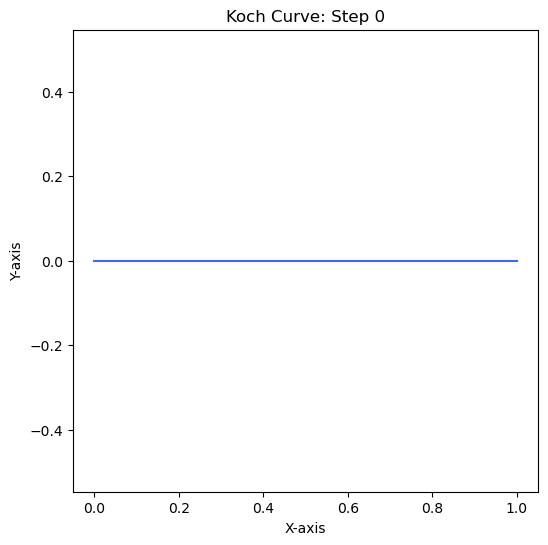
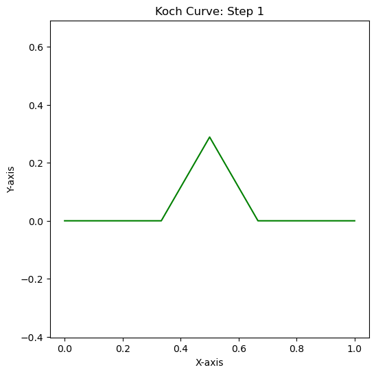
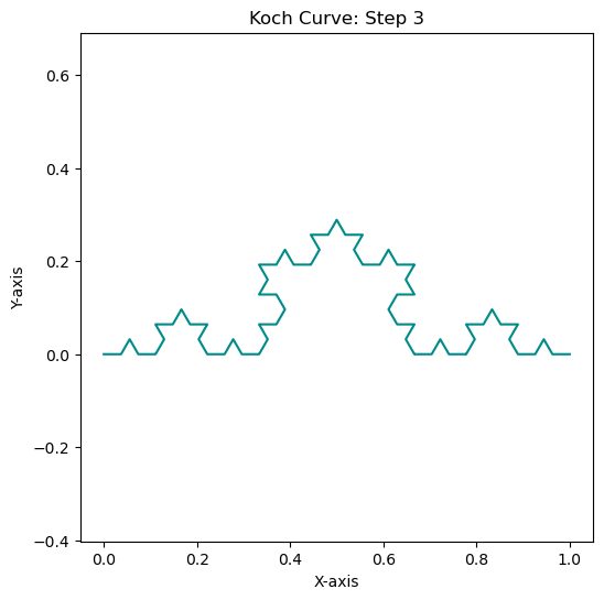
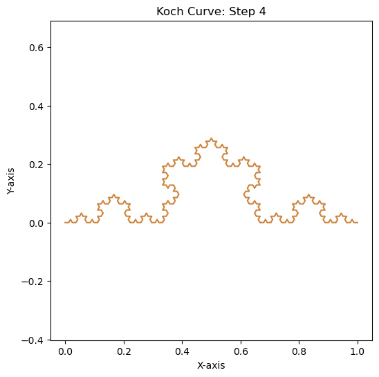
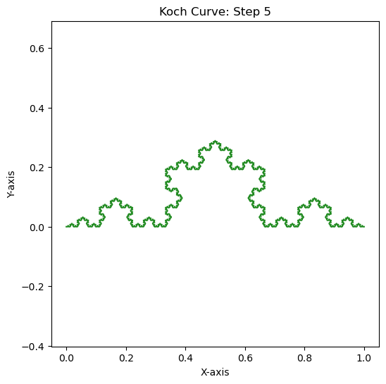
Example 3: The Koch Curves#
Show code cell source
# Example
x_user = np.array([0, 1])
y_user = np.array([0, 0])
my_angle = 60
steps = 5

color_palette = ['RoyalBlue', 'Green', 'Red', 'DarkCyan', 'Peru', 'ForestGreen']
# Generate the fractal pattern recursively
fractal = generate_fractal(x_user, y_user, steps, my_angle)
fractal.reverse()
for i, curve in enumerate(fractal):
    plt.figure(figsize=(6, 6))
    plt.title(f"Koch Curve: Step {i}")
    plt.xlabel("X-axis")
    plt.ylabel("Y-axis")
    plt.axis('equal')
    plt.grid(False)
    color = color_palette[i % len(color_palette)]
    plt.plot(curve[0], curve[1], color=color)
plt.show()

Interactive Exploration of the Koch Curve#
The following code snippet presents an interactive Koch curve. This allows you to observe the effect of changing the iteration step (recursion depth) on the complexity of the fractal. By adjusting the slider, you can witness the gradual increase in detail and self-similarity with each iterative step. This interactive exploration offers valuable insight into the generation process of recursive fractals like the Koch curve.
Attention
To access this interactive visualization, you’ll need a proper coding environment. Popular options include Binder, Jupyter Lab, and Google Colab, which provide the necessary tools to run the code behind the plot.
To launch the interactive environment, simply click the rocket icon () at the top of the page. This will open your chosen environment and allow you to execute the interactive plot.
Show code cell content
def color_random():
  """Returns a random color from a predefined list."""
  color_list = [
    'xkcd:midnight blue',      # A very dark blue
    'xkcd:bordeaux',           # A deep red wine color
    'xkcd:forest green',       # A dark green
    'xkcd:eggplant',           # A dark purple
    'xkcd:maroon',             # A dark red-brown
    'xkcd:navy blue',          # A dark blue
    'xkcd:dark olive',         # A dark greenish-brown
    'xkcd:indigo',             # A deep blue-violet
    'xkcd:charcoal',           # A dark gray
    'xkcd:dark plum',          # A deep purple
    'xkcd:dark teal',          # A dark blue-green
    'xkcd:dark brown',         # A dark brown
    'xkcd:royal purple',       # A dark purplish-blue
    'xkcd:pine green',         # A dark forest green
    'xkcd:chocolate',          # A dark brown
    'xkcd:midnight purple',    # A very dark purple
    'xkcd:dark forest green',  # A very dark green
    'xkcd:dark navy',          # A very dark blue
    'xkcd:dark fuchsia',       # A dark purplish-pink
    'xkcd:dark grass green',   # A dark green
    'xkcd:dark royal blue',    # A dark bluish-purple
    'xkcd:dark indigo',        # A very dark blue-violet
    'xkcd:scarlet',            # A red shade
    'xkcd:dark gold',          # A dark yellow
    'xkcd:dark lime green'     # A dark lime green
  ]
  return random.choice(color_list)


def create_line_fractal(steps: int):
    """
    Create a Koch Snowflake.

    Parameters:
    steps (int): The number of steps for the fractal generation.
    """

    # Prepare initial points for the line
    x_user = np.array([0, 1])
    y_user = np.array([0, 0])
    my_angle = 60
    color = color_random()
    # Generate the fractal pattern recursively
    fractal = generate_fractal(x_user, y_user, steps, my_angle)
    fractal.reverse()
    plt.figure(figsize=(6, 6))
    plt.title(f"Koch Curve Generation: Step {steps}")
    plt.xlabel("X-axis")
    plt.ylabel("Y-axis")
    plt.axis('equal')
    plt.grid(False)
    plt.plot(fractal[-1][0], fractal[-1][1], color=color)


def update_plot(steps):
    """update the plot"""
    create_line_fractal(steps)
    plt.show()
# Create a slider
steps_slider = widgets.IntSlider(min=0, max=5, step=1, description='Steps:', value=2)

# Use the slider to interact with the update_plot function
widgets.interact(update_plot, steps=steps_slider)
<function __main__.update_plot(steps)>
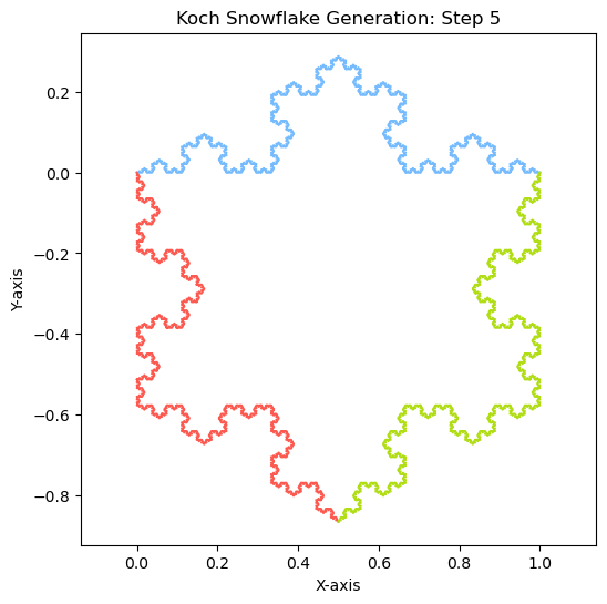
The Crystallization of the Koch Snowflake#
In this section, we explore the captivating process of constructing the Koch snowflake fractal. Unlike the Koch curve, which emerges from a single line, creating the snowflake demands a more complex approach. Initially, we transform one side of the triangle into a Koch curve. Then, by applying rotations and reflections, we efficiently construct the remaining two sides, ultimately achieving the snowflake’s intricate structure.
Once again, we combine the previously defined functions with a new function capable of rotating and optionally reflecting these curves to effectively generate the Koch snowflake. This new function, which takes the desired number of iterations as input, begins with an initial line segment as a side of an equilateral triangle and transforms it into a Koch curve through recursion. By applying this function twice more, it generates the other two sides of the snowflake through rotation and reflection. Once completed, the function plots the curves for visualization, and voila! Our virtual snowflake is crystallized for all to admire.
But the excitement doesn’t end there! We also offer an interactive version, where you can adjust the recursion depth with a slider and observe the snowflake unfold in real-time. This interactive experience provides a profound understanding of how this intricate fractal takes shape.
Show code cell source
def rotate_line(x_points: np.array, y_points: np.array, phi: float, cx: float, cy: float, reflect_across_x_axis=False) -> tuple:
    """
    Rotate a line around a given point by a certain angle, and optionally reflect it across the x-axis.

    Parameters:
    x_points (np.array): The x-coordinates of the points on the line.
    y_points (np.array): The y-coordinates of the points on the line.
    phi (float): The angle of rotation in degrees.
    cx (float): The x-coordinate of the point around which to rotate.
    cy (float): The y-coordinate of the point around which to rotate.
    reflect_across_x_axis (bool): Whether to reflect the line across the x-axis. Default is False.

    Returns:
    tuple: The x and y coordinates of the rotated (and optionally reflected) points on the line.
    """
    # If reflection across the x-axis is requested
    if reflect_across_x_axis:
        y_points = -y_points  # Reflect the y-coordinates across the x-axis

    # Convert angle from degrees to radians for numpy functions
    phi_rad = np.radians(phi)

    # Translate points to the origin
    x_translated = x_points - cx
    y_translated = y_points - cy

    # Perform rotation
    x_rotated = x_translated * np.cos(phi_rad) - y_translated * np.sin(phi_rad)
    y_rotated = x_translated * np.sin(phi_rad) + y_translated * np.cos(phi_rad)

    # Translate points back
    x_rotated += cx
    y_rotated += cy

    return x_rotated, y_rotated

def create_snowflake(steps: int):
    """
    Create a Koch Snowflake.

    Parameters:
    steps (int): The number of steps for the fractal generation.
    """
    # Prepare initial points for the line
    x_user = np.array([0, 1])
    y_user = np.array([0, 0])
    my_angle = 60

    # Generate the fractal pattern recursively
    fractal = generate_fractal(x_user, y_user, steps, my_angle)
    fractal.reverse()
    x_fractal = np.array(fractal[-1][0])
    y_fractal = np.array(fractal[-1][1])
    rotated_fractal1 = rotate_line(x_fractal, y_fractal, -60, 0, 0, True)
    rotated_fractal2 = rotate_line(x_fractal, y_fractal, 60, 1, 0, True)
    plt.figure(figsize=(6, 6))
    plt.title(f"Koch Snowflake Generation: Step {steps}")
    plt.xlabel("X-axis")
    plt.ylabel("Y-axis")
    plt.axis('equal')
    plt.grid(False)
    plt.plot(fractal[-1][0], fractal[-1][1], color='xkcd:sky blue')
    plt.plot(rotated_fractal1[0], rotated_fractal1[1], color='xkcd:coral')
    plt.plot(rotated_fractal2[0], rotated_fractal2[1], color='xkcd:yellowish green')

STEPS = 5
create_snowflake(STEPS)
plt.show()
Please play the video below to see the Koch Snowflake animation.
Show code cell source
# Configure matplotlib to correctly use ffmpeg on a local machine.
from IPython.display import HTML
import matplotlib
matplotlib.rcParams['animation.writer'] = 'ffmpeg'
matplotlib.rcParams['animation.ffmpeg_path'] = 'C:\\S.I.A.V.A.S.H\\Python\\Tools\\ffmpeg.exe'


def animate_snowflake(steps: int):
    """
    Create a Koch Snowflake.

    Parameters:
    steps (int): The number of steps for the fractal generation.
    """
    # Clear plots
    plt.clf()

    # Prepare initial points for the line
    x_user = np.array([0, 1])
    y_user = np.array([0, 0])
    my_angle = 60

    # Generate the fractal pattern recursively
    fractal = generate_fractal(x_user, y_user, steps, my_angle)
    fractal.reverse()
    x_fractal = np.array(fractal[-1][0])
    y_fractal = np.array(fractal[-1][1])
    rotated_fractal1 = rotate_line(x_fractal, y_fractal, 0, 0, 0, False)
    rotated_fractal2 = rotate_line(x_fractal, y_fractal, -60, 0, 0, True)
    rotated_fractal3 = rotate_line(x_fractal, y_fractal, 60, 1, 0, True)
    plt.title(f"Koch Snowflake Generation: Step {steps}")
    plt.xlabel("X-axis")
    plt.ylabel("Y-axis")
    plt.axis('equal')
    plt.xlim(-0.2, 1.2)
    plt.ylim(-0.95, 0.35)
    plt.grid(False)
    plt.plot(rotated_fractal1[0], rotated_fractal1[1], color='xkcd:sky blue')
    plt.plot(rotated_fractal2[0], rotated_fractal2[1], color='xkcd:coral')
    plt.plot(rotated_fractal3[0], rotated_fractal3[1], color='xkcd:yellowish green')


fig = plt.figure(figsize=(6, 6))

ani = animation.FuncAnimation(fig=fig, func=animate_snowflake, frames=6, interval=1000)

anim = ani.to_html5_video()
plt.close(fig=fig)

HTML(anim)
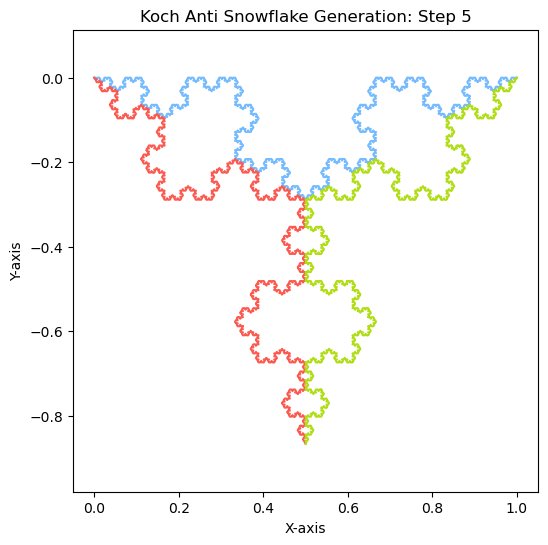
The Villain of Fractals#
After exploring the captivating construction of the Koch snowflake, let’s turn our attention to its evil twin, the Koch anti-snowflake. This variation offers a contrasting method to achieve fractal complexity. While the Koch snowflake builds intricate detail through iterative addition, the Koch anti-snowflake achieves a similarly complex form through a process of subtraction. Each iteration of the anti-snowflake removes equilateral triangles from the center of each side, resulting in a hollowed-out structure with a unique aesthetic. Despite this differing approach, the Koch anti-snowflake retains the self-similar and recursive properties that are hallmarks of fractals. In fact, its development showcases how complexity can emerge from both positive and negative space manipulation. The resulting form, with its minimalist, lace-like quality, offers a compelling counterpoint to the dense intricacy of the traditional Koch snowflake.
The exciting news? Just like its counterpart, the Koch anti-snowflake emerges from the same wellspring of code! We can conjure this fascinating fractal form by leveraging the same function we built for the Koch snowflake, with just a small tweak. No dark magic required! All it takes is a simple flip of a boolean parameter within the function, inverting the reflection, and bam! The dark side of the fractal world.
Show code cell source
def create_anti_snowflake(steps: int):
    """
    Create a Koch anti-snowflake.

    Parameters:
    steps (int): The number of steps for the fractal generation.
    """
    # Prepare initial points for the line
    x_user = np.array([0, 1])
    y_user = np.array([0, 0])
    my_angle = 60

    # Generate the fractal pattern recursively
    fractal = generate_fractal(x_user, y_user, steps, my_angle)
    fractal.reverse()
    x_fractal = np.array(fractal[-1][0])
    y_fractal = np.array(fractal[-1][1])
    rotated_fractal1 = rotate_line(x_fractal, y_fractal, 0, 0, 0, True)
    rotated_fractal2 = rotate_line(x_fractal, y_fractal, -60, 0, 0, False)
    rotated_fractal3 = rotate_line(x_fractal, y_fractal, 60, 1, 0, False)
    plt.figure(figsize=(6, 6))
    plt.title(f"Koch Anti Snowflake Generation: Step {steps}")
    plt.xlabel("X-axis")
    plt.ylabel("Y-axis")
    plt.axis('equal')
    plt.grid(False)
    plt.plot(rotated_fractal1[0], rotated_fractal1[1], color='xkcd:sky blue')
    plt.plot(rotated_fractal2[0], rotated_fractal2[1], color='xkcd:coral')
    plt.plot(rotated_fractal3[0], rotated_fractal3[1], color='xkcd:yellowish green')

STEPS = 5
create_anti_snowflake(STEPS)
plt.show()
Please play the video below to see the Koch Anti-Snowflake animation.
Show code cell source
def animate_anti_snowflake(steps: int):
    """
    Create a Koch anti-snowflake.

    Parameters:
    steps (int): The number of steps for the fractal generation.
    """
    # Clear plots
    plt.clf()

    # Prepare initial points for the line
    x_user = np.array([0, 1])
    y_user = np.array([0, 0])
    my_angle = 60

    # Generate the fractal pattern recursively
    fractal = generate_fractal(x_user, y_user, steps, my_angle)
    fractal.reverse()
    x_fractal = np.array(fractal[-1][0])
    y_fractal = np.array(fractal[-1][1])
    rotated_fractal1 = rotate_line(x_fractal, y_fractal, 0, 0, 0, True)
    rotated_fractal2 = rotate_line(x_fractal, y_fractal, -60, 0, 0, False)
    rotated_fractal3 = rotate_line(x_fractal, y_fractal, 60, 1, 0, False)
    plt.title(f"Koch Anti Snowflake Generation: Step {steps}")
    plt.xlabel("X-axis")
    plt.ylabel("Y-axis")
    plt.axis('equal')
    plt.grid(False)
    plt.plot(rotated_fractal1[0], rotated_fractal1[1], color='xkcd:sky blue')
    plt.plot(rotated_fractal2[0], rotated_fractal2[1], color='xkcd:coral')
    plt.plot(rotated_fractal3[0], rotated_fractal3[1], color='xkcd:yellowish green')


fig = plt.figure(figsize=(6, 6))
ani = animation.FuncAnimation(fig=fig, func=animate_anti_snowflake, frames=6, interval=1000)

anim = ani.to_html5_video()
plt.close(fig=fig)

HTML(anim)
Tip
The fractal dimension \(D\) can be calculated using the similarity dimension formula:
where \(N\) is the number of self-similar pieces, and \(S\) is the scaling factor.
For both the Koch snowflake and the Koch anti-snowflake, \(N = 4\) (since each segment is divided into 4 self-similar pieces) and \(S = 3\) (each segment is scaled down by a factor of 3). Plugging these values into the formula gives:
One intriguing property of fractals is their non-integer dimensions. Unlike traditional geometric shapes, fractals exist in a space between dimensions, showcasing complexity at every scale. This unique property allows fractals to infinitely reproduce their patterns, creating endlessly intricate structures.
Interactive Visualization of the Koch Snowflake and Anti-Snowflake#
To enhance our exploration of the Koch snowflake and Koch anti-snowflake, let’s introduce interactivity to our visualization. This will not only boost engagement but also deepen our understanding of this captivating fractal!
To run the interactive plot smoothly, simply click on the rocket icon () at the top of the page to access the Binder or Google Colab environment.
Show code cell content
# Define a function to update the plot
def update_plot(steps):
    """update the plot"""
    create_snowflake(steps)
    plt.show()
# Create a slider
steps_slider = widgets.IntSlider(min=0, max=5, step=1, description='Steps:', value=5)

# Use the slider to interact with the update_plot function
widgets.interact(update_plot, steps=steps_slider)
<function __main__.update_plot(steps)>
Show code cell content
# Define a function to update the plot
def update_plot(steps):
    """update the plot"""
    create_anti_snowflake(steps)
    plt.show()
# Create a slider
steps_slider = widgets.IntSlider(min=0, max=5, step=1, description='Steps:', value=5)

# Use the slider to interact with the update_plot function
widgets.interact(update_plot, steps=steps_slider)
<function __main__.update_plot(steps)>
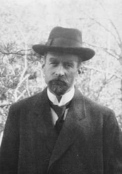
Fig. 5 Niels Fabian Helge von Koch (25 January 1870 – 11 March 1924) was a Swedish mathematician credited with giving his name to the famous fractal known as the Koch snowflake, one of the earliest described fractal curves. (Olof Edlund, Bookseller (SVAF), Public domain, via Wikimedia Commons).#
Summary: The Magic of Fractals#
In our Pythonic journey, we’ve witnessed the transformation of a simple line into the intricate Koch Snowflake through a series of magical spells cast by Python functions. These spells segmented lines, rotated points, and translated or reflected shapes, gradually unveiling the mesmerizing complexity of the fractal world.
Our adventure extended beyond creating a mere shape; it delved into the underlying mathematical principles, showcasing the power of iterative transformations. Each iteration built upon the last, revealing the captivating self-similarity inherent in fractals.
In conclusion, our journey showcased how abstract mathematical concepts can be translated into captivating visuals. We paid homage to mathematicians like Felix Hausdorff and Benoit Mandelbrot, who laid the groundwork for our understanding of fractals. Moreover, we explored how the concept of self-similarity permeates nature, from the intricate patterns of Broccoli to the delicate structures of Snowflakes or Anti Snowflakes.
As we conclude this adventure, we’re left with a profound appreciation for the magic of fractals and the potent sorcery of Python.
Published by Siavash Bakhtiarnia – May 16, 2024