Beyond Chance

Part 1: The Hidden Pattern in Every Dice Roll

Have you ever wondered what happens when you roll two dice? It seems like pure chance, but there’s a fascinating story behind the possible outcomes. Imagine you have a pair of regular six-sided dice, each face with a different number, just waiting to be tossed.

The key here is fairness. Each face of a die has an equal chance of landing face-up. When rolling two dice together, the possibilities multiply, resulting in 6 x 6 = 36 total possible outcomes. For example, you could get a 3 on one die and a 4 on the other.

However, not all sums of these rolls are equally likely. Sums like 2 (achieved only with a 1 on each die) and 12 (achieved only with a 6 on each die) are less probable because there’s only one way to get them. On the other hand, sums like 7 (achieved with several combinations such as 1 and 6, or 3 and 4) are more likely.

Now, this wouldn’t be much of a story without some data, right? Imagine how exciting it would be to plot these probabilities on a graph. We can leverage the power of Python and its libraries to simulate rolling dice as many times as we want and visualize the outcomes.

import random
import matplotlib.pyplot as plt
from collections import Counter

def simulate_dice_rolls(attempts):
    return [sum(random.randint(1, 6) for _ in range(2)) for _ in range(attempts)]

sums_possibilities = range(2, 13)

def plot_distribution(sums_possibilities, sums_distributions):
    plt.bar(sums_possibilities, sums_distributions, color='b')
    plt.xlabel('Sum of Dice')
    plt.ylabel('Probability')
    plt.title('Probability Distribution of Sums when Rolling Dice')
    plt.grid(False)
    plt.show()

Example 1: Throwing Two Dice 10 Times

Let’s kick off with a modest attempt: rolling two dice just 10 times and visualizing the distribution of their sums.

# Example 1
attempts_1 = 10
sums_1 = simulate_dice_rolls(attempts_1)
sums_counts_1 = Counter(sums_1)
sums_distributions_1 = [sums_counts_1[i] / attempts_1 for i in sums_possibilities]

# Plot distribution for Example 1
plot_distribution(sums_possibilities, sums_distributions_1)

Now If you roll the dice only a few times, like 10 as we just did, the resulting distribution wouldn’t be as smooth as you might expect. It might not reveal any clear pattern due to the randomness of a small sample. This reflects the bumpy landscape of chance with a small number of trials.

Example 2: Throwing Two Dice 500 Times

Now let’s take it up a notch and throw them 500 times.

# Example 2
attempts_2 = 500
sums_2 = simulate_dice_rolls(attempts_2)

sums_counts_2 = Counter(sums_2)
sums_distributions_2 = [sums_counts_2[i] / attempts_2 for i in sums_possibilities]

# Plot distribution for Example 2
plot_distribution(sums_possibilities, sums_distributions_2)

With each roll, the landscape of probability begins to morph, smoothing out its rough edges and revealing its underlying structure.

Example 3: Throwing Two Dice 100000 Times

Now, let’s push the boundaries further and throw the dice 100,000 times.

# Example 3
attempts_3 = 100000
sums_3 = simulate_dice_rolls(attempts_3)

sums_counts_3 = Counter(sums_3)
sums_distributions_3 = [sums_counts_3[i] / attempts_3 for i in sums_possibilities]

# Plot distribution for Example 3
plot_distribution(sums_possibilities, sums_distributions_3)

Behold the Empire State Building of probability! But why stop here? Let’s raise the stakes even further and add more dice to the mix.

# Roll the Dice Three Times
def simulate_dice_rolls_3times(attempts):
    return [sum(random.randint(1, 6) for _ in range(3)) for _ in range(attempts)]

sums_possibilities_3times = range(3, 19)

Example 4: Throwing Three Dice 100000 Times

Let’s see what happens when we throw three dice 100,000 times.

# Example 4
attempts_4 = 100000
sums_4 = simulate_dice_rolls_3times(attempts_4)

sums_counts_4 = Counter(sums_4)
sums_distributions_4 = [sums_counts_4[i] / attempts_4 for i in sums_possibilities_3times]

# Plot distribution for Example 3
plot_distribution(sums_possibilities_3times, sums_distributions_4)

As we introduce more dice into the equation, the complexity of the probability landscape deepens, offering new insights into the interplay of chance and pattern.

# Roll the Dice Four Times
def simulate_dice_rolls_4times(attempts):
    return [sum(random.randint(1, 6) for _ in range(4)) for _ in range(attempts)]

sums_possibilities_4times = range(4, 25)

Example 5: Throwing Four Dice 200000 Times

Let’s explore the realm of probability further by throwing four dice 200,000 times.

# Example 5
attempts_5 = 200000
sums_5 = simulate_dice_rolls_4times(attempts_5)

sums_counts_5 = Counter(sums_5)
sums_distributions_5 = [sums_counts_5[i] / attempts_5 for i in sums_possibilities_4times]

# Plot distribution
plot_distribution(sums_possibilities_4times, sums_distributions_5)

The bell curve’s elegant symmetry, peaking centrally and gently sloping towards its edges, offers a profound insight into how randomness coalesces into predictable patterns. It’s a striking demonstration of probability’s influence, showcasing how chance smoothens out over numerous attempts.

When rolling dice, it’s not just about the outcome at hand. It’s about appreciating the evolving story with each throw—a story where randomness gradually unveils a captivating, foreseeable pattern.

Part 2: From Playful Rolls to Universal Order

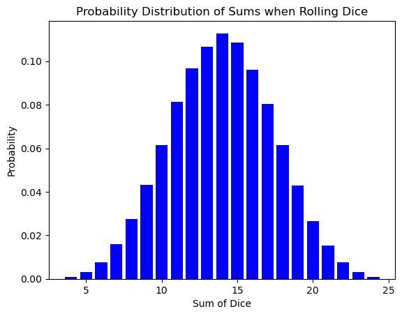
The bell curve of the dice sum distribution might seem like a simple quirk of rolling cubes. However, this very same shape pops up in a completely different arena: the world of atoms and energy!

Thermodynamics, the study of heat, work, and temperature, deals with systems containing a vast number of particles like atoms in a gas. Here, physicist Ludwig Boltzmann discovered that the distribution of energy levels in these tiny particles follows a similar bell-shaped curve. This is known as the Boltzmann distribution for overall energy, which also laid the groundwork for the Maxwell-Boltzmann Distribution. The Maxwell-Boltzmann Distribution takes the Boltzmann principle and applies it specifically to ideal gases. It focuses on the speeds (and related kinetic energies) of individual gas molecules. It tells you the probability of finding a molecule at a particular speed within the container at a specific temperature.

Tip

The Maxwell-Boltzmann distribution describes the speeds of atoms in an ideal gas container at a specific temperature. It’s not a uniform spread – most atoms have speeds around an average value, while fewer have very high or very low speeds. This reflects the range of kinetic energies atoms possess due to their constant motion and collisions. The distribution allows us to predict the probability of finding an atom at a particular speed within the container.

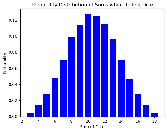
Here’s the exciting part: the number of times you roll the dice is analogous to the number of atoms in a system. Just like a single roll might result in an unlikely outcome (like double sixes), a single atom might have an unusual amount of energy or speed. But as the number of dice rolls increases, the randomness smooths out, revealing the underlying probability distribution.

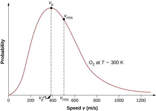
Fig. 1 The Maxwell-Boltzmann distribution of a gas at room temperature, from OpenStax [LMS16]

Imagine a giant container of gas with countless atoms bouncing around. While we can’t track the individual movements of each atom like we might with a few billiard balls (Newtonian mechanics shines there!), the sheer number of particles makes it impractical. However, probability comes to the rescue! By studying the overall behavior of the gas, like its temperature and pressure, we can use statistical methods (like the ones that govern dice rolls) to understand the average energy distribution of the atoms within.

Similarly, in a vast number of atoms (think Avogadro’s number!), the individual fluctuations in energy average out, and the familiar bell curve emerges. This distribution tells us how likely it is for an atom to have a particular energy level, just like the dice roll distribution tells us the likelihood of getting a specific sum.

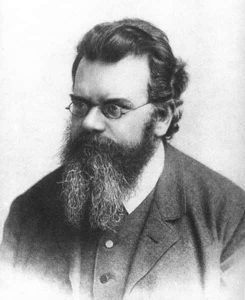
Fig. 2 Ludwig Boltzmann (Uni Frankfurt, Public domain, via Wikimedia Commons)

So, what does this all mean? It means the seemingly random world of dice rolls shares an interesting connection with the microscopic world of atoms. Both are governed by the same underlying principle of probability, where randomness averages out over a large number of events. The next time you pick up some dice, remember, you’re holding a tiny model of the universe, where chance and probability shape reality in fascinating ways.

Bibliography:

[LMS16]

Samuel J. Ling, William Moebs, and Jeff Sanny. University Physics Volume 2. OpenStax, 2016.

Published by Siavash Bakhtiarnia – March 28, 2024